What are the macroeconomic effects of reducing the central bank balance sheet size?
Based on research by Florencia S. Airaudo.
The Covid-19 crisis and the Federal Reserve balance sheet
To combat the COVID-19 crisis, the Federal Reserve implemented a stimulus program that included a Quantitative Easing (QE) program when short-term interest rates hit the zero lower bound (ZLB). The Federal Reserve’s balance sheet increased from 20 to 36% of GDP in two quarters due to asset purchases, primarily government bonds 1.
During this period, there was a significant fiscal expansion in the form of primary fiscal deficits and public debt-to-GDP ratios that had not been seen since World War II. The central bank’s purchase of government bonds played a vital role in sustaining demand for treasuries when private sectors, such as households, mutual funds, and the rest of the world, were selling their bond holdings. As a result of the 2020 QE program, one-fourth of the total US public debt was held by the Federal Reserve.
Figure 1: Central bank balance sheet in the US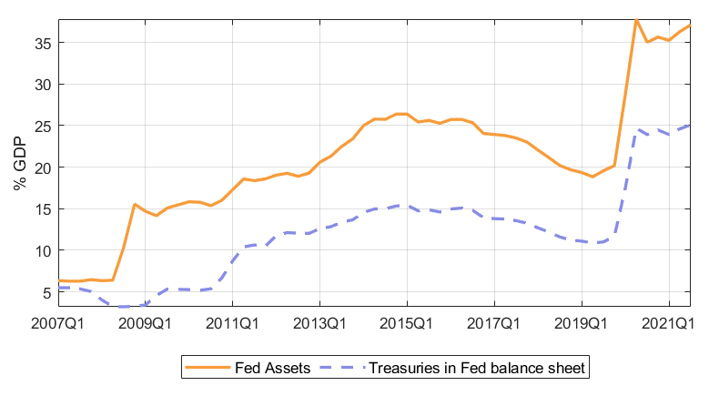
As the economy started to recover from the COVID-19 crisis, inflation far exceeded the target. In response, the Federal Reserve began to combine short-term interest rate increases with Quantitative Tightening (QT) to stabilize the inflation rate. QT involves the central bank stopping its purchase or selling of long-term public bonds in its portfolio, thereby reducing the size of its balance sheet. Despite the extension of this measure, there remains much uncertainty regarding the macroeconomic effects of QT.
A model of balance sheet policies and fiscal-monetary policy mix
In my ongoing work, I study the impact of QT on macroeconomic and financial variables such as inflation, public debt, and interest rates, considering the interaction between fiscal and monetary policies. To achieve this goal, I construct a regime-switching New Keynesian DSGE model calibrated to the US economy. This model is characterized by financial frictions and regime changes in the policy rules for conventional fiscal and monetary policies. I use the structural model to simulate the COVID-19 crisis and the policy responses and to investigate different QT policies.
The main finding of the paper is that the macroeconomic impact of QT hinges on how public debt is stabilized, whether through fiscal surpluses or inflation. When the fiscal authority adjusts taxes to stabilize the debt, QT can successfully reduce inflation, even with smaller increases in short-term interest rates. However, when there is no appropriate fiscal framework to stabilize the government debt, QT has little effect on inflation.
The DSGE model used in this paper comprises five agents: households, financial intermediaries, firms, the central bank, and the government. The fiscal authority issues long and short-term bonds, while the central bank issues reserves. The model incorporates market segmentation in the public debt market and a leverage constraint for financial intermediaries, similar to Elenev et al. (2021). Market segmentation implies that only households and the central bank purchase long-term public bonds, while only financial intermediaries invest in short-term bonds and reserves. These frictions break in the arbitrage condition between long and short-term public bonds, leading to real effects of QE and QT.
The central bank implements both conventional monetary policy and QE. The former involves using a Taylor rule for the short-term interest rate, the return on short-term public bonds, and reserves. Meanwhile, QE entails the central bank purchasing long-term government bonds from households and issuing reserves to financial intermediaries. The government follows a fiscal rule for taxes. The conventional policy rules switch between three regimes, as in Bianchi and Melosi (2017): monetary-led, fiscally-led, and ZLB. In the monetary-led regime, the fiscal authority adjusts the primary fiscal surplus to stabilize the public debt, while the central bank sets the short-term interest rate to stabilize inflation. In contrast, the fiscally-led regime involves the fiscal authority failing to adjust the fiscal surplus adequately to stabilize the debt, leading to the monetary authority allowing inflation to deviate from the target to stabilize debt in real terms. Finally, the ZLB regime represents a crisis regime where the monetary authority is constrained. The economy experiences recurrent regime switches, with endogenous transitions to and from the ZLB regime.
QE works through two channels: the increase in bank reserves and deposits, and the reduction in the long-term yield due to central bank intervention. Households rebalance their portfolio, selling long-term bonds for deposits due to the fall in long-term yields. Households’ wealth increases due to the portfolio revaluation effect, leading to higher consumption. The fall in savings returns generates a substitution effect from savings to consumption. As a result, QE raises aggregate demand, but the impact on output and inflation depends on the fiscal-monetary policy mix.
Crisis simulation and QT programs under different regimes
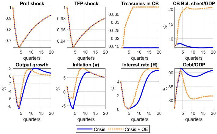
I calibrate the model for the US economy and simulate the COVID-19 crisis and policy response. The crisis is a result of negative demand and supply shocks 2. Figure 2 displays the mean simulated variables for the first 20 periods without QE (continuous blue line) and with QE (dotted orange line). Output growth drops to a low of -8.8p.p. in the fourth period, and debt-to-GDP rises. The short-term interest rate falls and reaches the ZLB.
I show that a QE program that increases the central bank’s balance sheet by 13p.p. of GDP reduces the persistence of the crisis. Output rebounds two quarters earlier compared to a scenario without QE, leading to a shorter duration of the ZLB regime. However, QE also has inflationary effects. During the crisis, prices fall by 2.5p.p. less with QE than without it. In the recovery, inflation reaches a peak of 8.4%. Without QE, inflation would still have overshot the target but at 6.9%.
Public debt-to-GDP decreases rapidly after the output and price recovery, and it falls even more under the QE program due to three reasons. First, QE increases central bank profits transferred to the treasury. Second, the debt service falls. And third, the faster recovery triggers a fall in government spending driven by the automatic stabilizers. These three factors allow the government to issue less debt during the crisis than in a counterfactual scenario without the QE program.
Figure 2: Simulated crisis with and without a QE program
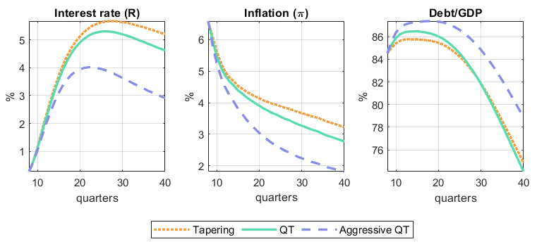
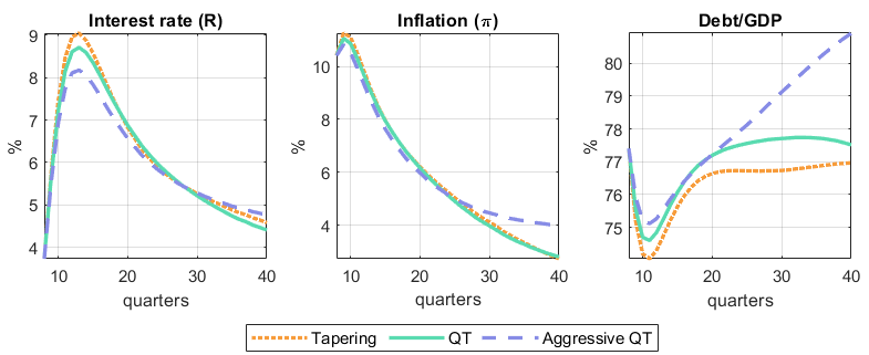
The study investigates the impact of the central bank’s balance sheet size on inflation, output, and debt dynamics during the crisis recovery. Different strategies are analyzed, including maintaining the enlarged size after the crisis (tapering), decreasing the balance sheet size by letting mature bonds run off (QT), and a faster reduction through selling bonds (Aggressive QT).
When the central bank does QT, it leads to a rise in long-term yields and a drop in bond prices. This shift prompts people to save more instead of consuming, which reduces demand and output. Additionally, there is an increase in public debt issuance due to higher debt service from rising interest rates, lower central bank remittances to the treasury, and an increase in the primary fiscal deficit caused by automatic stabilizers triggered by the output fall.
In the monetary-led regime, the increase in debt leads to an increase in taxes due to the fiscal rule. This exacerbates the decline in aggregate demand and disinflationary effects of QT. As a result, the inflation rate remains consistently lower with QT than with tapering. The difference in inflation tops at 1.5p.p., and this is achieved with lower increases in the short-term interest rate. With aggressive QT, the stance of the conventional monetary policy tool changes from contractionary to expansionary eight quarters before the tapering scenario.
Figure 3: QT in a monetary-led regime
In the fiscally-led regime, public debt increases actual and expected inflation, exacerbating the rise in yield spreads and mitigating the disinflationary effects of QT. In this regime, thus, there are no clear advantages in reducing the balance sheet size since it increases debt and spreads without helping to stabilize inflation.
Figure 4: QT in a fiscally-led regime
In sum, the macroeconomic impact of QT crucially depends on the fiscal-monetary mix. Reducing the balance sheet size in a monetary-led regime stabilizes inflation, but it may not be beneficial in a fiscally-led regime, as the stimulative effect of real negative interest rates and fiscal deficits counteract the negative demand shock generated by QT.
1 This rise in the ratios over GDP is mainly explained by asset purchases and not only by the fall in GDP. Assets in the central bank balance sheet increased from $4 to $8 trillion, while treasuries at the Federal Reserve increased from $2 to $6 trillion during the same time.
2 In the model, there is a strong shock to the Households’ discount factor (preference shock) and firms’ TFP.
Further Reading:
Airaudo, Florencia S. (2023). “Exit strategies from Quantitative Easing: the role of the fiscal-monetary policy mix”, working paper.
About the author:
Florencia Airaudo is a Ph.D. candidate in Universidad Carlos III de Madrid. She is interested in macroeconomics, monetary and fiscal theory and policy, international macroeconomics.
References:
Bianchi, F. and L. Melosi (2017): “Escaping the great recession,” American Economic Review, 107, 1030–58.
Elenev, V., T. Landvoigt, P. J. Shultz, and S. Van Nieuwerburgh (2021): “Can Monetary Policy Create Fiscal Capacity?” Tech. rep., National Bureau of Economic Research.